Two-Way Lookups in Excel

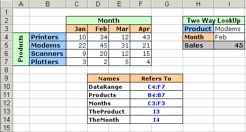
If you are a Excel user then invariably U must've have used the lookup functions of Excel, namely HLookUp() and VLookup(). For those who haven't: A lookup function is used to return a value from a given table by looking up another value in the same table. A simple example could be a discount table consisting of two columns, Purchase Amount & Discount. U can write a formula that uses VLookUp() to determine the discount rate for a given purchase amount.

Unfortunately the lookup functions in Excel are only appropriate for one-way lookups. There is no inbuilt worksheet function for performing a two-way lookup. Let me share my 2-way lookup formula with U.

Consider the table (refer to the figure) which displays the rather dismal monthly sales figures of various computer peripherals.

Objective:

To arrive at the Sales figure for Modems sold in Feb

Overview:

We shall make use of two functions Match() and Index() to create our two way lookup. Let me discuss briefly how these functions are used. For more detailed info look up the Excel help file.

Match(value_to_lookup, lookup_array, match_type): Returns the relative position of an item in an array that matches a specified value in a specified order. Value_to_lookup is the value you want to match in lookup_array. Lookup_array is a contiguous range of cells containing possible lookup values. Match_type specifies the matching criteria to be used. If match_type is 0, MATCH finds the first value that is exactly equal to value_to_lookup.
Index(array, row_num, column_num): Returns the value of an element in a table or an array, selected by the row and column number indexes. Array is a range of cells. Row_num selects the row in array from which to return a value. Column_num selects the column in array from which to return a value. INDEX returns the value in the array (cell) at the intersection of row_num and column_num.

My 2-Way lookup formula:

=INDEX(DataRange, MATCH(TheProduct,Products,0), MATCH(TheMonth,Months,0))

This is the formula in Cell I5.

Explanation:

MATCH(TheProduct,Products,0) will look up the value of the range TheProduct in the array Products and will return the position of the first occurrence of the value. If TheProduct is Feb then the above call will return 2 as Feb occurs at the second position in our array (Jan, Feb, Mar, Apr)

Similarly MATCH(TheMonth,Months,0) will look up the value of the range TheMonth in the array Months and will return the position of the first occurrence of the value. If TheMonth is Modems then the above call will return 2 as Modems occurs at the second position in our array (Printer, Modems, Scanners, Plotters)

Hence the above formula reduces to: =INDEX(DataRange, 2, 2) which returns the value of cell in the Range DataRange which occurs at the intersection of the 2nd Row and 2nd Column i.e 45. Yahoooooo!!!

For Advanced users:

Now the formula will return an error in case the Product or Month does not exist in the array. So let us use IsError() and If() to arrive at a more refined formula which will return 0 if either Product or Month does not exist in the Array.

=IF(ISERROR(INDEX(DataRange, MATCH(TheProduct,Products,0), MATCH(TheMonth,Months,0))),0,INDEX(DataRange, MATCH(TheProduct,Products,0), MATCH(TheMonth,Months,0)))